Graphing Cubic functions

Properties of Cubic’s

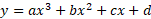
Cubic functions are identified by the fact that have an x term which is cubed. The general format for a cubic equation is:

This can also be in a factorised form which still has the capability to be graphed without expanding as the process is a simple substation in most cases.

Cubic functions differ to quadratic functions in that the graph will always cross the x axis, this is because there is at least one real root in the equation.

Local minimum and maximum

Local minimum point refers to the point in which the point on the graph has a horizontal tangent of 0 slope. The local maximum is the same, the difference between the two points is that it indicates if the graph continues down the y-axis or up the y-axis dependant on the sign of the value.

The term local in this case refers to the local area of the graph as unlike other graphs, Cubic’s will continue forever and cannot have an absolute maximum or minimum and so the term local is used.

Since a min and max point is simply the tangent at zero, we can use differentiation to determine a tangent point value at any x value. When we find the derivative, we actually want to ask the reverse question of when the tangent is zero what x value is that. The following steps will be taken to determine the value of the local min and max points:

• Differentiate the general cubic function to get a general quadratic equation
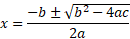
• Use the quadratic equation within the quadratic formula to get the x values of the local minimum and maximum. (This works by setting the resultant quadratic equation to zero to find the roots)
• Use the second derivative of the original equation to determine if the point is a min or max point based on the discriminates value.
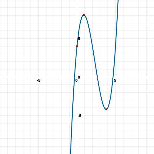
• Find additional points to help plot the graph such as the y-intercept (x = 0).

Example

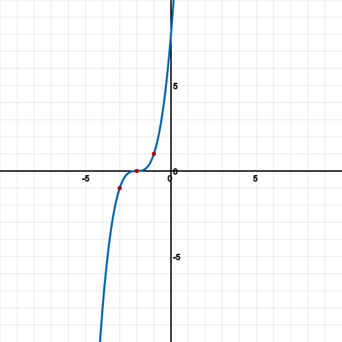
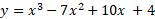
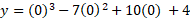
Find the local minimum and maximum of the cubic function f(x) = x³ – 7x² + 10x + 4

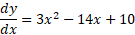
Step 1) Differentiate the equation:

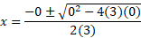
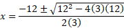
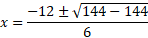
Step 2) Input this quadratic into the quadratic equation:

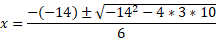
The discriminant is a none zero number and so there will be 2 answers for the x value and so a minimum and maximum will be present.

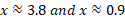
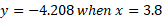
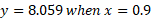
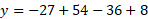
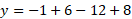
The Y value for the above points can be found simply by putting these specific x values back into the cubic equation:

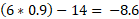
Step 3) find the second derivative of the quadratic equation and input the x values we just found:

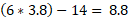
Now we know that for x at 3.8, the second derivative is positive meaning that this is a local minimum because the graph is set to go positive in the y axis on either side.

We also know that for x at 0.9, the second derivative is negative meaning that this is a local maximum because the graph is set to go negative in the y axis on either side.

Step 4) Find more values to help graph the equation.

The first easy one to graph is x = 0 as with most graphs.

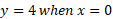
You may also choose points closest to the nearest integer of the min and max points. So, in this case x = 4 and x = 0. We already had x = 0 so x = 1 could work too.

So, plotting the points gives the following:

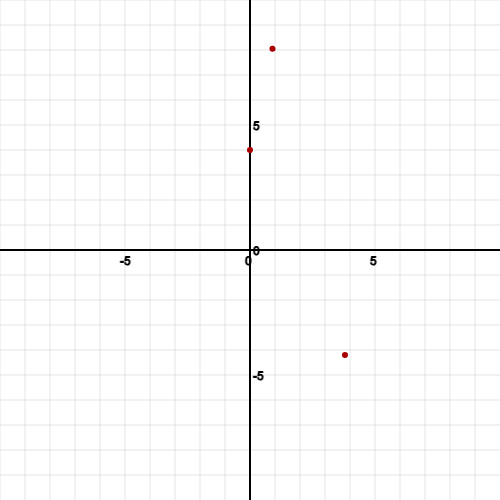
Connecting the graph should result in the following cubic:

Saddle point

A saddle point is a cubic with just one real root in which one point at the graph has a tangent slope of 0.

You use the same methods above when finding min and max points but the discriminant will always be zero for a saddle point. This means only one x value from the quadratic formula.

Example

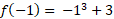
Find the slope of the tangent line equal to zero for the cubic function: f(x) = x³ + 3

First differentiate the function:

Now substitute this into the quadratic formula:

We didn’t have to use the quadratic formula here because knowing that 3x² = 0, then x would have to be zero anyway but it’s good to visualise how zero is the answer and the fact there is only one answer instead of 2 answers indicating this is indeed a saddle point.

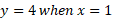
Substituting x = 0 back into the original cubic function gives a y value of 3. So when x = 0, y = 3. This is our first point.

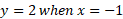
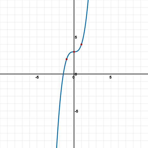
To graph this function, we can take an x point at either side of this saddle point and work out the y value.

The two values would be 1 and -1.

You could use additional points such as -2 and 2 for more accuracy or even fractional x values but this should be enough to graph:

Factorised form

Graph the equation: f(x) = (x + 2)³

When in factorised form such as this it can be rewritten into the form below:

When in this form it can be easier to work out what any y value is when we substitute an x value as we can just complete the equation.

We need to find points to plot on the graph, we need to know the point in which the graph curves and if it has a minimum, maximum or saddle point. It may also not have a point in which the gradient of the curve is zero and so we would need to know that too.

To find any points where the gradient is zero, we need to expand the factorised form to then use the methods mentioned before:

Now we can find the first derivative of the above expression:

Using the derived expression, we can use the quadratic formula to find the roots and determine where the graph will have any x values where the gradient of the tangent line equals zero.

We now know that when x = -2, y = 0. We also know how this graph should look as it has just one point meaning a saddle point, it should rise and stop then rise again.

We can now calculate additional points such as x = -3 and x = -1 because these are close to the saddle point:

When x = -3, y = -1

When x = -1, y = 1

We should now have enough points to graph the equation, you could plot more using the same method for better accuracy.