Binomial and Normal distributions

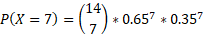
Binomial distributions

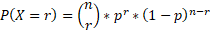
The above equation represents the binomial distribution equation and can be used to work out probabilities that satisfy specific characteristics.

X is binomially distributed when there are two outcomes, such as success and failure, hence the binomial term. The probability for success has to be the same each trial and so probability involving no replacement would not work with this.

So, for the above equation:

n = number of trials

r = number of successes

p = probability of success

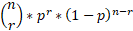
This can also be written as the following:

With the same attributes applying.

The number of trials could technically be represented by probability trees however with large amounts of trials this would be hard to draw and so the above equations are easier to follow.

A large data set however would also take a long time to calculate and so most calculators have cumulative distribution functions (cdf) and probability distribution functions (pdf) built into with the same variable options in the equations above and will provide the same result. This is found within the menu section.

You can find probabilities for a range of values in the form of inequalities. For example P(X < 7). This would mean all probabilities summed together for the successful outcomes within that range. A range of values would require using cumulative distribution function on the calculator.  

Example

1. The probability that a bus arrives at a particular stop on time is 0.65. The arrival time is independent each day. The bus comes to the same stop every day.
   1. Calculate the probability the bus arrives on time no more than 19 times in a 28-day period
   2. Calculate the probability the bus arrives on time exactly half the days in a 14-day period.

a) This question provides the information that we have multiple events each with late or not late (success or failure) and each event is independent. So, this can use binomial distribution.

Using this for the first part we can say that X is binomially distributed with the following parameters:

The specific probability we need to find is no more than 10 days in a 28-day period:

This is equal to:

We can input this data into the cumulative distribution function (cdf) on a calculator but if this was written in formula form it would be the following:

As you can see doing all these calculations individually would get quite complex and time consuming which is why a calculator would be needed:

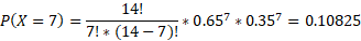
b) The second part of the question will have a different binomial distribution value as the days have changed from 28 to 14 but the method is the same:

The specific probability we need to find is exactly half the 14 days which is 7:

This can be calculated using the binomial probability distribution function (pdf) on a calculator or using the formula:

Normal distributions

Just like binomial distribution, normal distribution has its own notation to indicate that the random variable X is normally distributed with 2 values describing the data’s variance and mean.

μ = Mean

σ² = Variance

σ = Standard deviation

Normal distribution is a distribution of probabilities in equal directions of the mean with the most probable outcomes at the mean. It is used to determine probabilities within a range of values.

The normal distribution graph has horizontal asymptotes as it approaches zero but never touches it.

The total probability under the graph is equal to one.

The probability of a range of values is the area under the graph between two upper and lower bounds. Integration can be used to calculate this probability; however, the integral is non-elementary and incorporates the Gauss error function and so the best route of calculation is using a calculator instead.

The function of the graph, also known as the probability density function, is as follows:

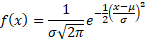
So, to work out the probability between two boundaries of the distribution graph you can integrate the above:

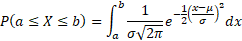
Again, a calculator does this for you but this is what the specific integral would look like.

On a calculator, choosing the normal cumulative distribution function, enter the corresponding values for the mean, standard deviation and the X values.

The mean lies in the centre of the distribution graph. The standard deviation can help us find specific probability data.

• Within 1 standard deviation of the mean, the total probability area is ≈ 68%.
• Within 2 standard deviations of the mean, the total probability area is ≈ 95%
• Within 3 standard deviations of the mean, the total probability area is ≈ 99.7%

3 standard deviations generally includes all the data that is required to work with but you can go much further in standard deviations to get specific results.

Example

1. The random variable X is normally distributed with a mean of 60 and a standard deviation of 10.
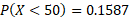
   1. Find P(X < 50)
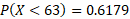
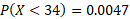
   2. Find P(34 < X < 63)

a) The question can be formatted into the normal distribution notation:

For the first part, X is less than 50, so entering these values into the normal cumulative distribution function with a lower bound of -99 (any lower bound large enough will suffice) we get the following result:

b) Just like part a, we use the same calculations except we need to convert the probability into two parts:

Standard normal distribution

The standard normal distribution can convert any normal distribution into a standard form where the mean is always 0 and the variance is 1 which means the standard deviation is also 1.

The standard normal distribution is represented by the value: Z

To convert a normal distribution to a standard normal distribution:

Using the Z value can be useful if a calculator only works with standard normal distributions.

The Z value is also useful to calculate the inverse of a normal distribution function if given an area and have to find the missing mean or standard deviation.

Because the standard normal distribution will always have a mean of 0 and a standard deviation of 1. It can be used to get the Z value and this can be substituted into the equation above to get any missing mean or standard deviation.

The inverse normal distribution function on a calculator can work out the value of a point on the graph given the area, the mean and standard deviation would 0 and 1 respectively as it will use the standard normal.

Example

1. The random variable X follows is normally distributed with a standard deviation of 4.
   1. If P(X < 13) = 0.9887, find the mean.
      
      

a) The mean is missing so we can first put the question into notation that is familiar

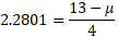
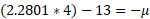
We can work out the Z value using the calculator as we know the area under the graph by the given probability:

As we now have the Z value, we can use the Z formula to find the mean for the specific probability distribution:

Solving for both mean and variance using simultaneous equations

Using similar methods above we can create two equations with two unknown variables being the mean and variance.

If we are given two probabilities for two different X values then we can create the simultaneous equations.

Example

1. Given the random variable X is normally distributed.
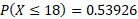
   1. If P(X < 18) = 0.2882 and P(X > 0.1152) Find the standard deviation and mean for this distribution.

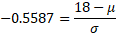
a) We have two missing variables we need to find so we will need to use simultaneous equations. The first step is to find the inverse normal or the probabilities given to get a Z value for both:

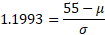
The second Z value can be calculated using the fact that 1 – 0.1152 is the same value, this is if the calculator only supports values less than a specific value.

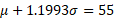
We now have what we need to formulate the simultaneous equation to solve for both variables:

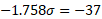
Rearrange:

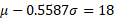
First solve for sigma by subtracting both equations:

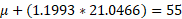
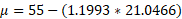
Now we can solve for mu by substituting sigma into one of the equations:

Normal approximations with Binomial distributions

Binomial distributions that meet specific characteristics can be approximated using a normal distribution as well.

A binomial distribution does not have a mean and variance so to find this for a binomial distribution you can do the following:

When representing binomial to normal we use Y:

Binomial distributions converted to normal distributions only work well if the probability is close to 0.5 and there is a large number of trials.

It can also work if np and nq are more than 5.

Binomial distributions are discrete and normal distributions are continuous, as mentioned before P(X = n) will always equal zero in a normal distribution. A continuity correction is needed to allow direct probabilities to be calculated.

The discrete random variable X is corrected to be continuous over a 0.5 either side. E.g. P(X = 1) = P(0.5 < X < 1.5) Allowing for the probabilities to be calculated in normal distribution.

Example

1. Given the random variable X is binomially distributed
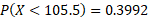
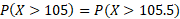
   1. find P(X > 105) using a normal approximation:

a) We can convert the binomial distribution to a normal distribution using the np and npq substitution for mean and variance:

The probability given will need to use a continuity correction:

We can convert to Z value and work out the normal distribution for this probability:

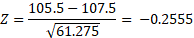
We can now input this as the upper bound and -100 as the lower bound on the calculator, this will give probability less than that value so to find more than this value we can subtract from 1: