Sorting Algorithms

Sorting algorithms are a fundamental part of computer science and are essential for organizing and managing data efficiently. The choice of the appropriate sorting algorithm is crucial because it can significantly impact the performance of an application.

Selecting the correct sorting algorithm depends on various factors, such as:

1. Size of the dataset: Some algorithms work well with small datasets, while others are more efficient with larger datasets.
2. Data distribution: The distribution and initial order of the data can affect the performance of some sorting algorithms.
3. Stability: Stable sorting algorithms maintain the relative order of equal elements, which can be crucial in specific applications.
4. In-place sorting: In-place algorithms use a constant amount of extra memory during the sorting process, making them more memory-efficient.
5. Adaptivity: Adaptive algorithms take advantage of existing order within the data to reduce the number of operations.

Standard Sorting Algorithm in Most Programming Languages

Many programming languages, such as Python, Java, and C++, use the Timsort algorithm as the default sorting algorithm. Timsort is a hybrid sorting algorithm derived from merge sort and insertion sort. It takes advantage of runs (already ordered subsequences) in the input data and is adaptive, stable, and performs well on real-world data.

Sorting algorithm complexities can be expressed using Big O notation, which describes the upper bound of the algorithm's growth rate. The most common complexities are:

1. O(n^2): Quadratic complexity, typical for elementary sorting algorithms such as bubble sort, insertion sort, and selection sort. These algorithms perform well for small datasets but become inefficient as the dataset size increases.

2. O(n*log(n)): Log-linear complexity, typical for more advanced algorithms such as merge sort, quicksort, and heapsort. These algorithms are more efficient for larger datasets.

3. O(n): Linear complexity, found in linear-time sorting algorithms such as counting sort, radix sort, and bucket sort. These algorithms are efficient for specific types of data but are not suitable for all data types.

Fastest Type of Sorting Algorithm: Quicksort

Quicksort is a highly efficient and widely used sorting algorithm, which employs a divide-and-conquer strategy. It works by selecting a 'pivot' element from the array and partitioning the other elements into two groups: those less than or equal to the pivot and those greater than the pivot. The process is then recursively applied to the sub-arrays, eventually resulting in a sorted array.

The average-case time complexity of quicksort is O(n*log(n)), where n is the number of elements in the array. The O-notation, also known as Big O notation, represents the upper bound of an algorithm's growth rate. It is used to describe the performance or complexity of an algorithm as a function of input size.

To understand how the O(n*log(n)) complexity comes into play for quicksort, let's consider a specific example:

Suppose we have an array of 8 elements: [5, 3, 9, 1, 6, 8, 2, 7]

In each step, quicksort will partition the array around the pivot, and for simplicity, let's assume the pivot selection always results in a balanced partition (i.e., the pivot element is the median). After each partition, the array will be split into two halves, and quicksort will be applied recursively to both halves.

Here's how the array will be partitioned in each step (with pivot elements in parentheses):

1. [5, 3, (1), 6, 8, 2, 7, 9]
2. [(1), 5, 3, 6, 8, 2, 7, 9] -> [(1), 3, 5, (2), 7, 8, 6, 9]
3. [(1), 3, 5, (2), 7, 8, 6, 9] -> [(1), 3, (2), 5, 7, 8, (6), 9]
4. [(1), 3, (2), 5, 7, 8, (6), 9] -> [(1), (2), 3, 5, (6), 7, 8, 9]

In this example, quicksort had to perform log2(8) = 3 levels of partitioning (with each level doubling the number of sub-arrays), and at each level, a total of n = 8 comparisons were made. Therefore, the total number of comparisons is:

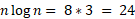
To use the O(n*log(n)) equation for quicksort, you can simply plug in the number of elements in the array (n) and calculate the product of n and log2(n). Keep in mind that this represents the average-case complexity, and the actual number of comparisons may vary depending on the input data and pivot selection strategy.

The lower the value of O(n*log(n)), the more efficient the algorithm. In the context of sorting algorithms, the Big-O notation represents the number of comparisons or operations performed in the worst-case scenario. The lower the number of comparisons, the faster the algorithm will perform, especially for larger datasets.

Similarly, for other notations like O(n^2) and O(n), they represent the number of comparisons or operations made in the worst-case scenario. For example:

• O(n^2) implies that the number of comparisons grows quadratically with the input size. Algorithms with this complexity, such as Bubble Sort or Insertion Sort, tend to be less efficient for large datasets.
• O(n) implies that the number of comparisons grows linearly with the input size. Linear-time algorithms, such as Counting Sort (for specific cases) or Radix Sort, can be more efficient for certain types of data.

Comparing different algorithms' complexities helps in understanding which one may perform better for a specific problem or dataset.

Example quicksort code in JavaScript: